This is the first of a three-part post, where we’re going to look at how you can create an appointment system using Google Forms and Sheets and with the use of Apps Script, how you it will update the available times on the forms and how it will send automate confirmation emails to those making the appointments.
I’ve used this system for parents evening meetings, but it could be adapted for any area that need appointments.
In this part, we’ll look at setting up the sheet, getting it ready to make the forms and appointment sheets.
Part 2, will look at the code used to create the forms and sheets.
Part 3, will look at the code that sends the parents a confirmation email and that adds the form responses to the appointment sheets.
HOW THE SYSTEM WILL WORK
- Parents receive an email inviting them to the parents’ evening and asking them to click on a link to choose an appointment time.
- They fill in a pre-filled in Google Form, where they just need to select an appointment time.
- The details are recorded on a Google Sheet, where there is a sheet per group with all the appointments.
- The time is removed from the Google Form, as it is now not available.
- The parent receives a confirmation email with the appointment details.
INITIAL SET UP
First, you will need the master documents:
Google Sheet – This will create the forms and also receive the appointments.

Google Forms – Blank masters. In this example, there are two as we have 2 possible time blocks for parents evening.
GOOGLE SHEET
In the Google Sheet there are 3 sheets:
students – This is where all the student and class information will be added.
Plus, this is where the pre-filled form links will be created.
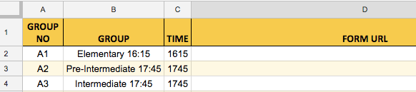
formLinks – This is a list of the classes and this is where the blank form URLs for each class will be added by the script.
toEmail – This is optional, but this is a sheet to catch any emails that weren’t sent if the daily quota has been exceeded. In my school, we have to send about 400 emails and with a Gmail account, you can only send 100 a day. So, we use this to send any that didn’t go out.

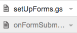
Finally, there are 2 script files, one to set up the forms and the sheets, and the other is to record the appointments and send the confirmation emails, when a form is submitted.
GOOGLE FORMS
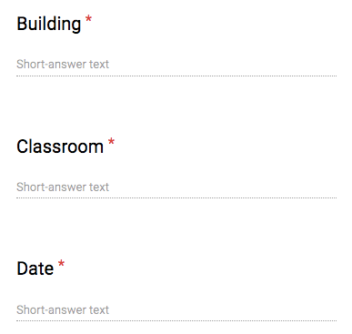
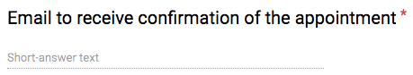
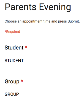
The master forms contain the details about the student, class, etc. All these fields except the appointment time will be pre-filled out. Make sure, all the fields are marked required.
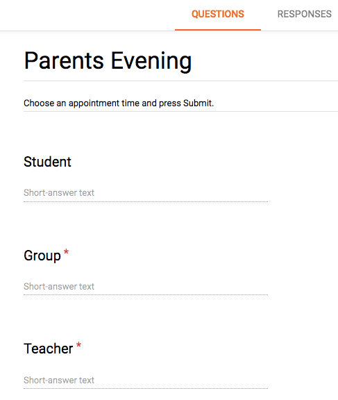
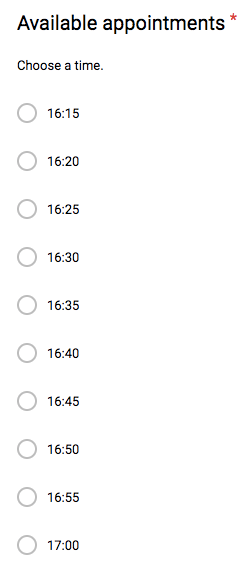
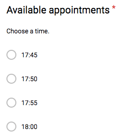
The only difference between the two forms, is the available times. One has from 16:15 and the other from 17:45.
SETTING UP THE SHEET
The first step is to add the list of your classes to the ‘formLinks’ sheet. Here, we have a group number, group name, and the time block the appointments will be at. The final column is left blank.
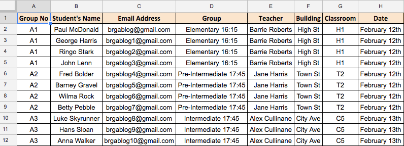
Now, add the students and class details on the ‘students’ sheet. The email address is the one which will receive the appointment confirmation email, so will usually be one of the parents. I’ve included building as we have classroom at different sites.
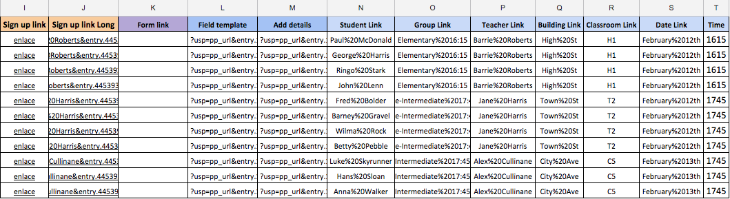
Columns I to T contain formulas, which take the above details and change it into a format ready for the pre-filled form URL, which will be shared with the parents. You’ll only need to set up the sheet with these formulas once.
Creating the pre-filled form links
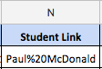
I’ll take you through the columns in the order the form URL is created. So, first columns N to T, take the original details and clean it up so it’s ready to be added to the URLs. This is mainly necessary as URLs don’t like spaces in them as it can break the URL. So, we’ll need to substitute any spaces with the character code %20. A URL recognises this as a space. We’ll also trim the original data, in case any spaces how crept in.
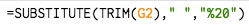
So, looking at column N, we write the following formula:
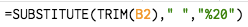
This gets the value in cell B2, removes any white spaces at the start or end of it, using the TRIM function, and then substitutes any spaces in the middle with the character %20. Here, we can see it’s taken the name Paul McDonald and added the %20 in the middle.
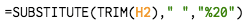
The formula is the same for each of the columns up until column S. Just change the reference cell each time.


In column T, add we’re going to check to see what time is in the group name and record it as a 1615 block or 1745 block. We do that by using the following formula:


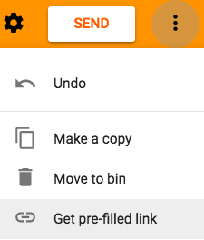
Now, we need to get the end of the URL, which will tell the form to pre-fill certain information. Open one of the form masters in edit mode and click on the 3-dot menu and select ‘Get pre-filled link’.
Fill in the fields with the field titles, e.g. Student, write STUDENT.
Then press “Get link”.

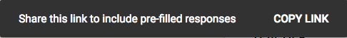
Click on “Copy link”. Unfortunately, the link is displayed like it used to be, so you’ll need to paste it somewhere, e.g. on a spare sheet in a Google Sheet.
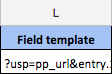
As you can see it’s extremely long! The part that interests us, is the part after where it says ‘viewform’, from and including the question mark, as this is the part which details which fields are to be filled out and what with. So, copy the URL from and including the question mark all the way to the end.

Then paste it in cell L2.
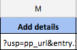
Now, we need to substitute the words we added in the fields (e.g. STUDENT) with the data on our sheet. We do that by using the SUBSTITUTE function. This has 3 parts, it gets the original text, looks for a term you want to replace, and states what you want to replace it with. The great thing is that they can be nested, so you can substitute several terms in one go.

=SUBSTITUTE(SUBSTITUTE(SUBSTITUTE(SUBSTITUTE(SUBSTITUTE(SUBSTITUTE(SUBSTITUTE($L2, “STUDENT”, $N2), “GROUP”, $02), “TEACHER”, $P2), “BUILDING”, $Q2), “CLASSROOM”, $R2), “DATE”, $S2), “EMAIL”, $C2)
Write this in cell M2.
Now we need to get the blank form URL for our group. These are stored in the formLinks sheet, so we can use a VLOOKUP function to look up the group name on the ‘students’ sheet and then look up that group on the formLinks sheet. See my post on using VLOOKUP.

=VLOOKUP(D2, formLinks!$B$2:$D$4,3,FALSE)
Write this in cell K2.
We then need to combine the blank URL and the fields URL together. We do that by using the CONCATENATE function and getting column K and M.
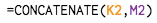
=CONCATENATE(K2, M2)
We write that in cell J2.
Finally, as we’re going to share this link in an email to the parents, it would be better to add a short link rather than this huge URL. So, we use the HYPERLINK function to get the long URL, and label it “link”.
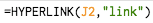
=HYPERLINK(J2,”link”)
Write it in cell I2 and you’ll see it creates a link called ‘link’.

Now, you’ll need to copy I2 to T2 down, so that there are formulas in all the rows of your data.
This may all seem rather complicated but once the sheet is set up, you don’t need to do it again. Now, the sheet’s ready to have the forms and appointment sheets made. See the next post for that!
Here you can make a copy of the Google Sheet.
Plus, here are the 2 master forms I’ve used: form1615, form1745
Here‘s bit more info on the SUBSTITUTE function.
Want to learn more about Google Workspace and Apps Script? The books below are available on Amazon. Just click on a book! (Affiliate links).


a


